gridgen

Tutorial

gridgen consists of some functions (commands) that allow you to:

create the 2d grid (grid2d)
create the 3d grid (grid3d)
compute the power spectral density (PSD) at each electrode (ecog)
fit the 3d grid onto the surface (fit)
- by correlating the morphology and/or functional values with the ECoG values (metric = parametric or metric = nonparametric)
- by finding the highest sum of the electrodes estimated from the morphology and/or functional values (metric = sum)
compare the results (matlab)

In addition, you need to pass the parameters for your analysis. Parameters are structured in a json format. A description of the parameters can be found in Parameters.

You can also generate an template json file with all the necessary parameters with the command:

gridgen parameters.json parameters

Then you need to populate the values in parameters. Note that each command requires different set of parameters. f.e.

gridgen parameters.json grid2d

only requires the parameter grid2d while the command:

gridgen parameters.json grid3d

requires the parameters grid3d, mri, initial (and possibly morphology and functional). This information is described in Parameters and gridgen will throw an error if the parametes are not complete.

grid2d

The first step is to create a 2d grid. This grid will only give us the electrode labels and no additional information (so, no information about electrode spacing). You can create a grid with the parameters (called parameters.json):

{
  "grid2d": {
    "n_rows": 4,
    "n_columns": 3,
    "direction": "TBLR",
    "chan_pattern": "chan{}"
    }
}

By convention, the wires are at the bottom. chan_pattern is used to generate the channel labels. chan{} will create chan1, chan2, chan3 and chan{:03d} will create chan001, chan002, chan003 (see Python string formatting).

The command

gridgen parameters.json grid2d

will create a file called grid2d_labels.tsv like this:

grid2d_labels.tsv

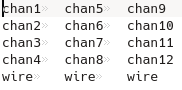
This file will be used by the other commands (ecog, grid3d, fit).

Note that you can modify this text file as you want (f.e. by moving the channels around, in case the grid labels are in a different order).

grid3d

After having created grid2d_labels.tsv, you can create a 3d grid, onto the smooth surface (convex hull, dura surface). You’ll need to pass additional parameters. At the minimum, you need to specifiy:

{
  "grid3d": {
    "interelec_distance": 3,
    "maximum_angle": 5
    },
  "mri": {
    "T1_file": "analysis/data/brain.mgz",
    "dura_file": "analysis/data/lh_smooth.pial"
  },
  "initial": {
    "label": "chan4",
    "RAS": [-47, -1, 3],
    "rotation": 0
  }
}

initial indicates which electrode should be used as starting point and you should specify the (rough) RAS coordinates of that electrode. The command

gridgen parameters.json grid3d

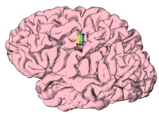
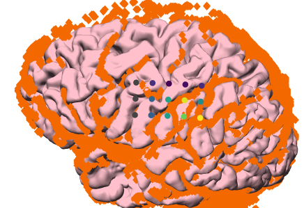
will look for the closest vertex on the smooth surface (start electrode). Starting from the start electrdoe (green), the locations for the other electrodes are created one at the time, according to this idea:

principles

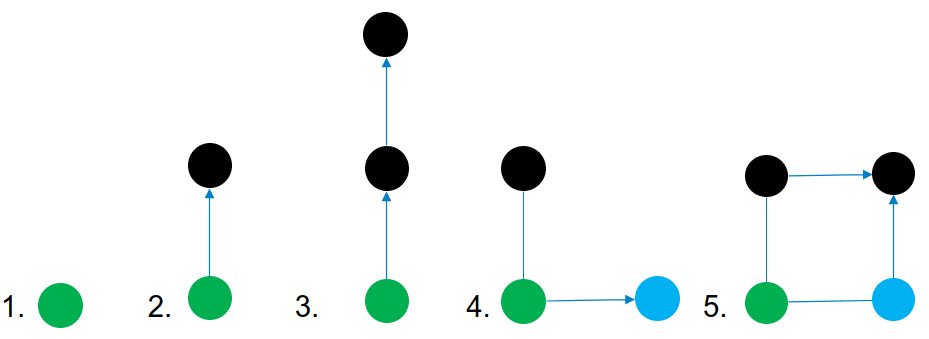
Start electrode (which is at the exact location as the vertex on the smooth surface, and with the same normal)
Find the next electrode (based on the normal of the start electrode and the rotation parameter, where 0 is roughtly upwards). The next electrode should also be on the smooth surface.
Continue finding the next electrode on the same column, following the same line (the position of the new electrode follows the normal from the green electrode and the first black electrode, until it touches the smooth surface or it reaches the maximum_angle).
Find electrodes along the rows. The angle between black-green and blue-green should be roughly 90° but not necessary.
Find the electrode at the intersection between the other two electrodes. The constraint is that the two arrows have the same length (but the angle might not be 90°).

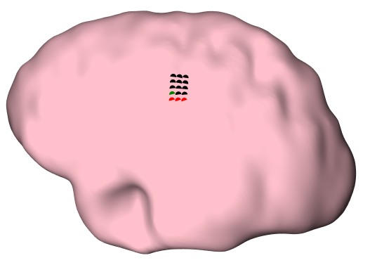
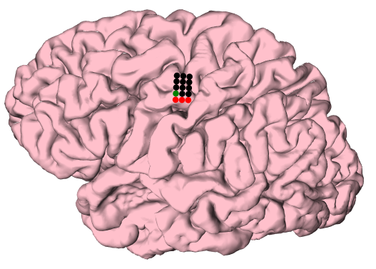
The output is a folder with:

electrodes.tsv : electrode locations in T1 space
electrodes.label : electrode locations for freeview
electrodes.fcsv : electrode locations for 3DSlicer
electrodes.html : interactive plot with electrode locations

which looks like this:

grid3d

Morphology (pial surface)

You can also add the pial surface. The plot will use the pial surface and will compute the morphology:

{
  "grid3d": {
    "interelec_distance": 3,
    "maximum_angle": 5
    },
  "mri": {
    "T1_file": "analysis/data/brain.mgz",
    "dura_file": "analysis/data/lh_smooth.pial"
    "pial_file": "analysis/data/lh.pial"
  },
  "initial": {
    "label": "chan4",
    "RAS": [-47, -1, 3],
    "rotation": 0
  },
  "morphology": {
    "distance": "ray",
    "penalty": 2
  }
}

which looks like:

grid3d

and it will compute the morphology:

grid3d morphology

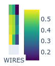
The distance can be:

ray : distance between electrode and the intersection of the normal of the electrode and the pial surface
minimum : distance between electrode and closest vertex on the pial surface
view : distance between electrode and closest vertex inside a cone (angle of the cone: 30°)
cylinder : distance between electrode and closest vertex inside a cylinder (electrode is the center) After computing the distance, you can specify penalty, which is the exponent when computing the penalty from the distance. Morphology = 1 / distance^penalty. More simply, 1 = activity decreases linearly with distance; 2 = activity decreases with the square of the distance.

distance can also be pdf, where the value associated with each electrode with the weighted sum of the distance of all the vertices on the pial surface, weighted by a gaussian 3d smoothing kernel. penalty in this case refers to the sigma of the 3D smoothing kernel.

Rotation

The orientation when rotation = 0 is roughly upwards (inferior-superior axis). It might not always follow this axis exactly (it’s just a convention), so try different rotation values to see the orientation that you want. You can then add rotation (in degrees, clockwise):

{
  "grid3d": {
    "interelec_distance": 3,
    "maximum_angle": 5
    },
  "mri": {
    "T1_file": "analysis/data/brain.mgz",
    "dura_file": "analysis/data/lh_smooth.pial"
    "pial_file": "analysis/data/lh.pial"
  },
  "initial": {
    "label": "chan4",
    "RAS": [-47, -1, 3],
    "rotation": 90
  },
  "morphology": {
    "distance": "ray",
    "penalty": 2
  }
}

grid3d rotation

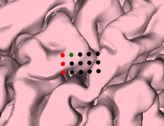
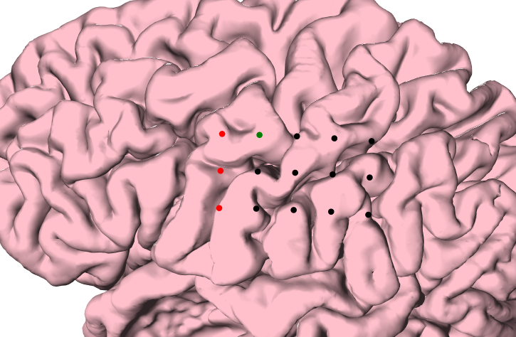
The start electrode is shown in green, the other electrodes are in black and the wires are in red.

Inter-electrode Distance

You can also change the distance between electrodes:

{
  "grid3d": {
    "interelec_distance": 10,
    "maximum_angle": 5
    },
  "mri": {
    "T1_file": "analysis/data/brain.mgz",
    "dura_file": "analysis/data/lh_smooth.pial",
    "pial_file": "analysis/data/lh.pial"
  },
  "initial": {
    "label": "chan4",
    "RAS": [-47, -1, 3],
    "rotation": 90
  },
  "morphology": {
    "distance": "ray",
    "penalty": 2
  }
}

grid3d interelec distance

Grid Rigidity

You can also modify the rigidity of the grid, which is controlled by the maximum_angle parameter (i.e. the maximum angle between two neighboring electrodes).

{
  "grid3d": {
    "interelec_distance": 10,
    "maximum_angle": 5
    },
  "mri": {
    "T1_file": "analysis/data/brain.mgz",
    "dura_file": "analysis/data/lh_smooth.pial",
    "pial_file": "analysis/data/lh.pial"
  },
  "initial": {
    "label": "chan4",
    "RAS": [-18, -81, -31],
    "rotation": 90
  },
  "morphology": {
    "distance": "ray",
    "penalty": 2
  }
}

grid3d grid rigidity

Functional Data (Angiogram)

In addition to the morphology (based on a mesh), you can calculate some metrics at each electrode based on a 3D MRI volume. The MRI volume can be an angiogram (which gives you the location of the blood vessels) or a t-map with activity at each voxel, so that you can combine fMRI results with the ECoG electrodes.

Angiogram

First, make sure that the angiogram is realigned to the T1 (see Preparation). Then you specify the parameters in functional. In this case, you only include voxels above 90 (all the voxels above the threshold are given a value of 1 and those below the threshold are given a value of 0). Then you compute the number of voxels in a sphere of a radius of 8mm around each electrode:

{
  "grid3d": {
    "interelec_distance": 10,
    "maximum_angle": 5
    },
  "mri": {
    "T1_file": "analysis/data/brain.mgz",
    "dura_file": "analysis/data/lh_smooth.pial",
    "pial_file": "analysis/data/lh.pial",
    "func_file": "analysis/data/angiogram.nii.gz"
  },
  "initial": {
    "label": "chan4",
    "RAS": [-47, -1, 3],
    "rotation": 90
  },
  "morphology": {
    "distance": "ray",
    "penalty": 2
  },
  "functional": {
    "threshold": 90,
    "metric": "sphere",
    "kernel": 8
  }
}

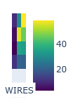
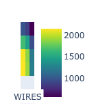
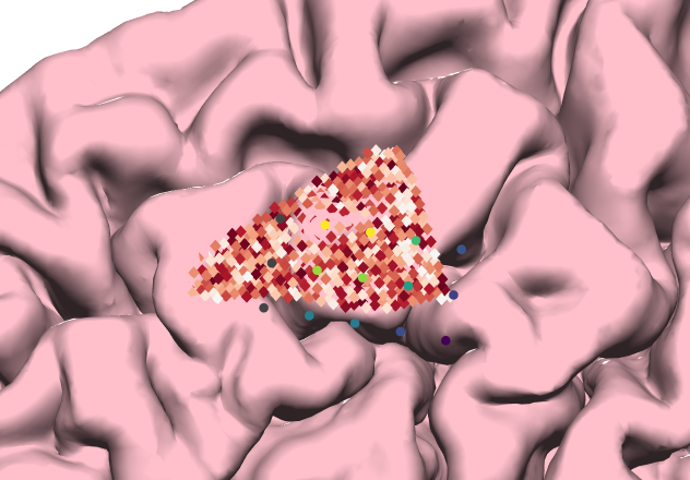
The output will also return a plot called functional.html which shows the angiogram and the values for each electrode:

grid3d angiogram

fMRI

If you have the results of the fMRI as t-maps, you can compute the weighted 3D average, based on a 3D gaussian weighting kernel, as described in Piantoni, G. et al. “Size of the spatial correlation between ECoG and fMRI activity.” NeuroImage 242(2021): 118459 .

Note that we do not binarize the MRI in this case, so threshold should be set to null.

{
  "grid3d": {
    "interelec_distance": 5,
    "maximum_angle": 5
    },
  "mri": {
    "T1_file": "../analysis/data/brain.mgz",
    "dura_file": "../analysis/data/lh_smooth.pial",
    "pial_file": "../analysis/data/lh.pial",
    "func_file": "../analysis/generated/tmap.nii.gz"
  },
  "initial": {
    "label": "chan4",
    "RAS": [-32, 25, 12],
    "rotation": 90
  },
  "morphology": {
    "distance": "ray",
    "penalty": 2
  },
  "functional": {
    "threshold": null,
    "metric": "gaussian",
    "kernel": 8
  }
}

Because there is no fMRI available for this patient, the fMRI tmap is just random numbers above zeros in one region.

grid3d gaussian

Another useful metric is inverse in which the value at each electrode is the sum of the voxels around the electrode, weighted by the inverse of the distance.

ecog

You can compute the PSD in the high-frequency range with this parameters.json:

{    
  "ecog": {
    "ecog_file": "analysis/generated/ecog.eeg",
    "freq_range": [60, 90]
  }
}

which generates

grid2d_ecog.tsv : values of the power spectrum per electrode
grid2d_ecog.html : plot of the estimated activity of the power spectrum

Note that these values are not projected on the 3D grid or surface yet.

fit

You can fit the most likely 3d grid location based on the morphology of the cortex and the functional maps (especially angiogram), so that they match the ECoG values. After running gridgen parameters.json grid2d and gridgen parameters.json ecog, you can use the following parameters:

{
  "grid3d": {
    "interelec_distance": 10,
    "maximum_angle": 5
    },
  "mri": {
    "T1_file": "analysis/data/brain.mgz",
    "dura_file": "analysis/data/lh_smooth.pial",
    "pial_file": "analysis/data/lh.pial",
    "func_file": "analysis/data/angiogram.nii.gz"
  },
  "initial": {
    "label": "chan4",
    "RAS": [-47, -1, 3],
    "rotation": 90
  },
  "morphology": {
    "distance": "ray",
    "penalty": 2
  },
  "functional": {
    "threshold": 100,
    "metric": "sphere",
    "kernel": 8
  },
  "fit": {
    "morphology_weight": 1,
    "functional_weight": -1,
    "method": "brute",
    "ranges": {
      "x": [-10, 5, 10],
      "y": [-10, 5, 10],
      "rotation": [-10, 5, 10]
      }
  }
}

There are two methods available (see below). The fitting procedure will correlate the ECoG values with those computed with a combination of morphology and functional maps. You can specify the direction of the correlation:

"morphology_weight": 1 means that the higher the morphology values, the higher the ECoG values are expected to be (because the vertices are closer to the electrode),
"functional_weight": -1 means that the higher the functional values, the lower the ECoG values are expected to be (because the blood vessels suppress the ecog activity). Morphology and functional values are normalized between 0 and 1 beforehand.

The fitting procedure will run for a while. Here we specify a very sparse range value (the step value is 5) for quicker computation.

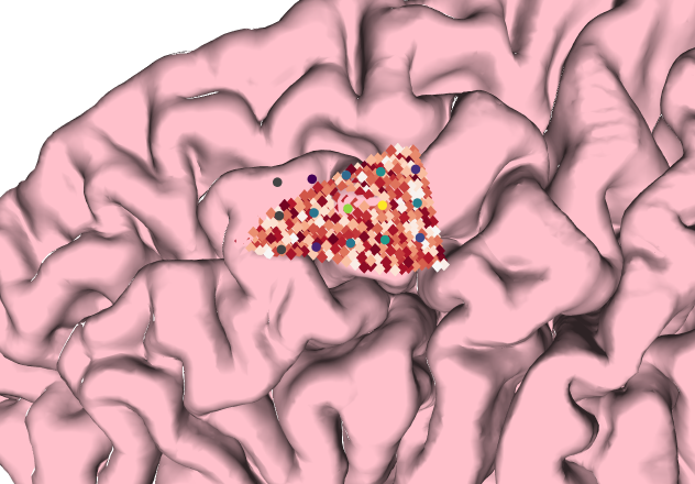
The results show:

parameters.json : summary of the parameters used for the fit
results.json : summary of the results to recompute the grid and fit
electrodes.tsv : electrode locations for the best fit in T1 space
electrodes.label : electrode locations for the best fit for freeview
electrodes.fcsv : electrode locations for the best fit for 3DSlicer
projected.html : interactive plot with electrode locations for the best fit (with ECoG values)
morphology.html : the values for each electrode based on morphology of the pial surface
functional.html : the values for each electrode based on functional MRI
merged.html : the combined values of functional and morphology values

Brute Force

Compute the model at each combination of the values in the range. The ranges are specificied with [start point, step size, end point]. It runs in parallel and at the end it runs the simplex method as well (for increased accuracy).

  "fit": {
    "method": "brute",
    "ranges": {
      "x": [-10, 1, 10],
      "y": [-10, 1, 10],
      "rotation": [-10, 1, 10]
      }
  }

Simplex (Nelder-Mead)

Fitting procedure is based on the Nelder-Mead method. You should specify the step sizes in each direction, then it computes the value at each node of the simplex:

You should specify the size of the simplex in each direction with steps:

  "fit": {
    "method": "simplex",
    "steps": {
      "x": 5,
      "y": 5,
      "rotation": 4
      }
  }

There are no bounds, so it can get out of the start position, if it can find a better fit. It’s a good idea to run:

gridgen --log debug parameters.json grid2d

So that you see the steps and values computed at each node of the simplex.

fit (sum metric)

You can also fit the electrode grid in such a way that the electrodes capture the highest functional activity. To compute this, we calculate the functional value at each electrode and we sum the values over all the electrodes. The grid location with the highest sum of values is the output of this procedure. In this case, we do not need to compute ECoG beforehand.

Here is a minimum parameter file:

{
  "grid3d": {
    "interelec_distance": 5,
    "maximum_angle": 5
    },
  "mri": {
    "T1_file": "analysis/data/brain.mgz",
    "dura_file": "analysis/data/lh_smooth.pial",
    "func_file": "analysis/generated/tmap.nii.gz"
  },
  "initial": {
    "label": "chan4",
    "RAS": [-27, 30, 13],
    "rotation": 70
  },
  "functional": {
    "threshold": null,
    "metric": "sphere",
    "kernel": 8
  },
  "fit": {
    "metric": "sum",
    "method": "simplex",
    "steps": {
      "x": 5,
      "y": 5,
      "rotation": 1
      }
  }
}

The results should look like this:

In principle, you can also use the morphology values. The morphology and functional values are then merged based on morphology_weight and functional_weight. Values are not normalized between 0 and 1 in this case, so you can adjust the parameters to adjust for the differences in magnitude.

    "morphology_weight": 1e5,
    "functional_weight": 1,

In practice, it’s tricky to find the right balance between the two weights.

fit sum

Notes

The json files used to compute the analysis of this tutorial can be found here

This site is open source. Improve this page.